This quick-start tutorial demonstrates how to configure the MOEA/D algorithm and apply it to the DTLZ2 problem with two objectives. Furthermore, it is demonstrated how numerical results can be reported and how the visualization of the final population can be performed. The complete source code for this tutorial can be found in the Projects module: y2025.SoftwareX_JECDM.QuickStart1 (framework’s version at least 1.7.0). In what follows, the relevant commented code blocks are presented, and the expected results are visualized for convenience. Before starting, however, a list of necessary imports for this example can be found below:
The overview of the source code:
Let us start with defininf the criteria/objectives:
// The following line instantiates 2 criteria using a factory-like method.

Criteria C = Criteria.constructCriteria(
        "C", // denotes a prefix for criteria names ("C0", "C1")
        2, // denotes the number of criteria to instantiate
        false //indicates that the criteria are cost-type.
);Code language: PHP (php)
Now, we can define the problem-specifica data:
// Now, let us instantiate a DTLZ2 packed in a bundle-like class. It comprises various auxiliary data, e.g., the Pareto front bounds, and delivers the evaluation procedure, while also providing default reproduction and initialization phases (SBX and PM operators; random vectors initialization; see the method's code for further information).

DTLZBundle dtlz2 = DTLZBundle.getBundle(
        Problem.DTLZ2, // the problem id
        C._no, // the problem dimensionality
        DTLZBundle.getRecommendedNODistanceRelatedParameters(Problem.DTLZ2, C._no) // the number of
        // distance-related variables (10 + no. objectives - 1):

        // Alternatively, you can also supply your own operator constructors, as shown in the following example:
        // (problem, M, D) -> new SBX(1.0d, 20.0d), // probability = 1.0; distribution index = 20.0
        // (problem, M, D) -> new PM(1.0d / (double) (D + M), 20.0d) // probability = 1 / (the number of decision variables for this problem = 12); distribution index = 20.0)
);Code language: JavaScript (javascript)
Then, we can proceed to instantiating the MOEA/D algorithm:
// Now, instantiate the MOEA/D method, using the factory-like static method (it is recommended to examine other similar static methods in this class):

MOEAD moead = MOEAD.getMOEAD(
        true, // This flag indicates that MOEA/D will be parameterized to dynamically update its internal data on the known Pareto front bounds during optimization (false = the data is fixed and derived from the bundle; in the case of DTLZ2, the bounds are [0, 1] intervals; they are used primarily to properly normalize objectives when evaluating solutions given the scalarizing functions employed
        new L32_X64_MIX(0), // the random number generator instantiated with a seed of 0 for reproducibility,
        // The decomposition-based methods are implemented in a way that they abstract from the concrete definition of the scalarizing functions employed (see the IGoal interface). We will use the regular PBI functions with the aggregating factor of 5.0:
        GoalsFactory.getPBIsDND(  // get PBI functions whose reference points' positions are determined using the Das and Dennis' method
        C._no, // the number of objectives
        29, // the number of divisions for the Das and Dennis' method (will result in the population size of 30)
        5.0d), // the aggregating factor of 5.0:
        dtlz2, // problem bundle (delivers by default dedicated operators, etc.; these can also be supplied by
        // using other static methods of the MOEA/D class)
        new Euclidean(), // similarity/distance definition used to build goals' neighborhood
        // (the interface's isLessMeaningCloser() implementation dictates the interpretation of measurements)
        10 // the neighborhood size
);Code language: PHP (php)
Now, we can execute the method. Two means of doing that are presented:
// The EA can be executed manually by calling its init and step methods. The former is associated with the 0th generation, during which mainly an initial population is constructed and evaluated. The step method executes a regular generation process that involves parent selection, reproduction, evaluation, and survival of the fittest, among other steps. Note that the method requires providing the current generation number as the input. These generation numbers should start from 1, as 0 is reserved for the init step.

try
{
    moead.init();
    for (int g = 1; g < 300; g++)
        // Important note: the MOEA/D is implemented as a steady-state algorithm. It means that one generation
        // comprises a series of updates, each tackling a different optimization goal (equivalent of an inner
        // loop). A timestamp passed via the step method can comprise the current generation number and the
        // steady-state number. Thus, the inner loop processing can be done in this way. The number of the
        // so-called steady-state repeats should be equal to population size, as, by default, one offspring
        // is constructed during the update (thus, the number of performance solution evaluations equals
        // the number of generations * the population size):
        for (int ssr = 0; ssr < moead.getPopulationSize(); ssr++)
            moead.step(new EATimestamp(g, ssr));

} catch (EAException e)
{
    throw new RuntimeException(e);
}

// Alternatively, a dedicated runner object can be used to perform the evolution. It is worth noting that it  can handle multiple EAs as well as coupling the simulation with visualization (note that the moead.getPopulationSize() parameter indicates the number of steady-state repeats to be performed within one generation)

/*IRunner runner = new Runner(new Runner.Params(moead, moead.getPopulationSize()));
try
{
    runner.executeEvolution(200);
} catch (RunnerException e)
{
    throw new RuntimeException(e);
}*/Code language: PHP (php)
The following piece of code accesses the specimens and prints the information on their objective and decision vectors:
// Now, let us print the population:

for (Specimen s : nsgaii.getSpecimensContainer().getPopulation())
{
    String sb = PrintUtils.getVectorOfDoubles(s.getEvaluations(), 3) + // objective vector (precision of three decimal places)
            " : " + // separator
            PrintUtils.getVectorOfDoubles(s.getDoubleDecisionVector(), 3); // decision vector (precision of three decimal places)
    System.out.println(sb);
}Code language: JavaScript (javascript)
Expected first lines of the console output:
0.000 1.002 : 1.000 0.514 0.484 0.508 0.499 0.496 0.514 0.479 0.496 0.490 0.518 0.504
0.036 1.002 : 0.977 0.489 0.513 0.508 0.495 0.488 0.514 0.478 0.526 0.498 0.519 0.504
0.074 0.999 : 0.953 0.490 0.506 0.510 0.508 0.497 0.482 0.473 0.496 0.516 0.489 0.504
0.115 0.995 : 0.927 0.514 0.505 0.508 0.495 0.497 0.482 0.479 0.496 0.490 0.489 0.504
0.158 0.989 : 0.899 0.517 0.487 0.507 0.500 0.511 0.482 0.479 0.501 0.494 0.505 0.507
Additionally, we can calculate the hypervolume attained by the final population and compare it with the easy-to-calculate optimum:
// We can also perform a simple performance assessment using a standard hypervolume metric.

HV.Params pHV = new HV.Params( // the parameterization of various objects in this framework is often conducted via an inner static class called Params, which is then passed via the constructor
        C._no, // the number of objectives considered
        dtlz2._normalizations, // functions used to normalize the input objective vectors into [0,1] hypercube
        ArrayUtils.getDoubleArray(C._no, 1.1d) // set the reference point (nadir) in the normalized space to [1.1, 1.1]
);

// Let us now instantiate the indicator:

IPerformanceIndicator indicator = new HV(pHV);
double hv = indicator.evaluate(nsgaii); // calculate the hypervolume based on the current state of the algorithm

// We can easily calculate the optimal hypervolume in this setting (1.1^2 - one fourth of a 1-radius disk):
double optimalHV = 1.1d * 1.1d - Math.PI / 4.0d;
System.out.println("HV = " + hv); // print the attained hypervolume
System.out.println("Optimal HV = " + optimalHV); // print the optimal hypervolume
System.out.println("Difference = " + (optimalHV - hv)); // print the differenceCode language: JavaScript (javascript)
Expected console output:
HV = 0.4076069855708936
Optimal HV = 0.4246018366025519
Difference = 0.01699485103165832
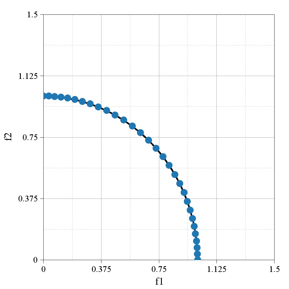
We can finally visualize the last population constructed by MOEA/D. It begins by creating the plot:
// Finally, let us visualize the constructed population using a 2D plot. We will use the Plot2DFactory class for this purpose, which allows for the quick instantiation of simple 2D plots. Note that this class features numerous static factory methods, enabling various customizations.

Plot2D plot2D = Plot2DFactory.getPlot(
        "f1", // label for the x-axis
        "f2", // label for the y-axis
        1.5d, // limit for both axes: [0; limit]
        1.2f, // auxiliary parameter for relative font rescaling (1.0 = default value)
        scheme -> scheme._colors.put(ColorFields.PLOT_BACKGROUND, Color.WHITE) // plot scheme adjuster can be
        // supplied via this argument; the plot look is mostly controlled by a Scheme object that can be altered
        // on the fly in this way; this piece of code sets the plot background color to white (transparent by default)
);Code language: JavaScript (javascript)
Then, a dedicated Frame object (extends the Java Swing’s Frame class) must be instantiated:
// The plot object is displayed using a dedicated Frame (extension of JSwing's Frame):

Frame frame = new Frame(
        plot2D, // plot to be displayed
        800, // plot width in pixels
        800 // plot height in pixels
);Code language: PHP (php)
After instantiating the plot and the frame, we can start preparing the data sets to be visualized:
// We can now supply the plot with data sets to be visualized. Note that it can only be done after bounding the plot with the frame. We will visualize the Pareto front and the final population (objective vectors).

ArrayList<IDataSet> dataSets = new ArrayList<>(2); // initialize an array of data sets
// Prepare the pareto front:
dataSets.add(
        // ReferenceParetoFront class provides simple methods for quickly instantiating straightforward Pareto
        // fronts to be displayed. Here, we ask for a concave spherical 2D front.
        ReferenceParetoFront.getConcaveSpherical2DPF(
                1.0d, // the radius of the sphere
                new LineStyle(0.5f, color.gradient.Color.BLACK) // line style (width and color)
        )
);

// Now, we can construct a data set representing the population. For this reason, we will use the primary way of instantiating data sets: a dedicated factory-like class, DSFactory2D.
dataSets.add(
        DSFactory2D.getDS(
                "Population", // the data set name
                new EASource(moead).createData(), // we need to provide objective vectors defined as double[][]
                // matrix; for this purpose, we will use an auxiliary data processor: EASource
                new MarkerStyle( // finally, we can define the marker style
                        3.0f, // marker size
                        ColorPalettes.getFromDefaultPalette(0), // color obtained from the default color palette (bluish)
                        Marker.CIRCLE // marker style
                )
        )
);

// The following line delivers the data sets to be displayed to the plot:
plot2D.getModel().setDataSets(dataSets);Code language: PHP (php)
The following piece of code displays the rendered plot:
// Finally, we can display the plot (ensure that the screen scaling in the OS is set to 1.0 for best outcomes; a different factor may result in visual artifacts):
frame.setVisible(true);Code language: JavaScript (javascript)
Lastly, this tutorial showcases how to create the plot’s screenshot that can be then used, e.g., in one’s publication:
// For this quick start tutorial, the screenshot of the plot is generated and stored. It can be accomplished in the following way:

Screenshot screenshot = plot2D.getModel().requestScreenshotCreation(
        1000, // screenshot width (independent to the current plot width)
        1000,  // screenshot height (independent to the current plot height)
        false, // do not use the alpha channel
        null // optional parameter that indicates that the plot will be clipped to its content by
        // removing the first/last columns/rows that match the given color (e.g., check Color.WHITE)
);

// Generating the screenshot is asynchronous. We need to wait by calling .await() on the provided synchronization barrier:

try
{
    screenshot._barrier.await();
} catch (InterruptedException e)
{
    throw new RuntimeException(e);
}

// Finally, we can use the following method to save the screenshot.

ImageSaver.saveImage(
        screenshot._image, // screenshot to be saved
        "D:" + File.separatorChar + "quickstart2", // file path (excludes the extension; alter it according to your computer specification and needs)
        "jpg", // file extension (only regular file types, e.g., bmp or jpg are supported; in the case of providing an unsupported extension, an error message will be printed)
        1.0f // image quality (1.0 = the best; not all extensions support this parameter)
);Code language: JavaScript (javascript)
The expected final render is provided below. Note the satisfactory performance in terms of distribution, which is often attributed to the decomposition-based methods.
Used imports:
import color.Color;
import color.gradient.ColorPalettes;
import criterion.Criteria;
import dataset.DSFactory2D;
import dataset.IDataSet;
import dataset.painter.style.LineStyle;
import dataset.painter.style.MarkerStyle;
import dataset.painter.style.enums.Marker;
import ea.EATimestamp;
import emo.aposteriori.moead.MOEAD;
import emo.utils.decomposition.goal.GoalsFactory;
import emo.utils.decomposition.similarity.lnorm.Euclidean;
import exception.EAException;
import exception.RunnerException;
import frame.Frame;
import indicator.IPerformanceIndicator;
import indicator.emo.HV;
import io.image.ImageSaver;
import plot.Plot2D;
import plot.Plot2DFactory;
import population.Specimen;
import print.PrintUtils;
import problem.Problem;
import problem.moo.dtlz.DTLZBundle;
import random.L32_X64_MIX;
import reproduction.operators.crossover.SBX;
import reproduction.operators.mutation.PM;
import runner.IRunner;
import runner.Runner;
import scheme.enums.ColorFields;
import utils.ArrayUtils;
import utils.Screenshot;
import visualization.updaters.sources.EASource;
import visualization.utils.ReferenceParetoFront;

import java.io.File;
import java.util.ArrayList;Code language: CSS (css)